Concept Drift: 8 Detection Methods

There is a wide range of techniques that can be applied for detecting concept drift. Becoming familiar with these detection methods is key to using the right metric for each drift and model.

In the article below, I review four types of detection methods: Statistical, Statistical Process Control, Time Window Based, and Contextual Approaches.

If you’re looking for an introduction to concept drift, I recommend checking out my post Concept drift in machine learning 101.

Statistical Methods

Statistical methods are used to compare the difference between distributions. In some cases, a divergence is used, which is a type of distance metric between distributions. In other cases, a test is run to receive a score.

Kullback–Leibler Divergence

Kullback–Leibler divergence is sometimes referred to as relative entropy. The KL divergence tries to quantify how much one probability distribution differs from another, so if we have the distributions Q and P where the Q distribution is the distribution of the old data and P is that of the new data we would like to calculate:

$KL(Q||P) = – displaystylesum_x{P(x)}*log(frac{Q(x)}{P(x)})$

* The “||” represents the divergence.

We can see that if P(x) is high and Q(x) is low, the divergence will be high.

If P(x) is low and Q(x) is high, the divergence will be high as well but not as much.

If P(x) and Q(x) are similar, then the divergence will be lower.

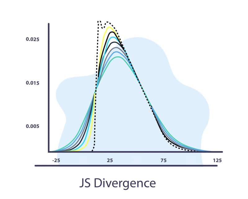
JS Divergence

Jensen-Shannon Divergence uses the KL divergence

$JS(Q||P) = frac{1}{2}(KL(Q||M) +KL(P||M))$

Where $M = frac{Q+P}{2}$ the mean between P and Q

The main differences between JS divergence and KL divergence are that JS is symmetric and it always has a finite value

Kolmogorov-Smirnov Test

The two-sample KS test is a useful and general nonparametric method for comparing two samples. In the KS test we calculate:
$D_{n,m}=sup_{x}|F_{1,n}(x) – F_{2,m}(x)|$

Where $F_{1,n}(x)$ is the empirical distribution function of the previous data with $n$ samples and $F_{2,m}(x)$ is the empirical distribution function of the new data with $m$ samples and $F_{n}(x) = frac{1}{n} displaystylesum_{i=1}^n I_{[- infty,x]}(X_{i})$. The $sup_{x}$ is the subset of samples x that maximizes $|F_{1,n}(x) – F_{2,m}(x)|$.

The KS test is sensitive to differences in both location and shape of the empirical cumulative distribution functions of the two samples. It is well suited for numerical data.

When to use Statistical Methods

The idea in the statistical methods section is to assess the distribution between two datasets.

We can use these tools to find differences between data from different timeframes and measure the differences in the behavior of the data as time goes on.

As for these methods, the label is not needed, and no additional memory is required; we can get a quick indicator for changes in the input features/output to the model. That would help us start investigating the situation even before any potential degradation in the model’s performance metrics. On the other hand, the lack of a label and disregarding memory of past events and other features could result in false positives if not handled correctly.

Statistical Process Control

The idea of statistical process control is to verify that our model’s error is in control. This is especially important when running in production as the performance changes over time. Thus, we would like to have a system that would send an alert if the model passes some error rate. Note that some models have a “traffic light” system where they also have warning alerts.

Drift Detection Method/Early Drift Detection Method (DDM/EDDM)

The idea is to model the error as a binomial variable. That means that we can calculate our expected value of the errors. As we are working with a binomial distribution we can mark =npt and therefore $sigma = sqrt{frac{p_{t}(1-p_{t})}{n}}$.

DDM

Here we can raise:

• A warning when $p_{t}+sigma_{t}ge p_{min} +2sigma_{min}$
• An alarm when $p_{t}+sigma_{t}ge p_{min} +3sigma_{min}$

Pros: DDM shows good performance when detecting gradual changes (if they are not very slow) and abrupt changes (incremental and sudden drifts).

Cons: DDM has difficulties detecting drift when the change is slowly gradual. It is possible that many samples are stored for a long time, before the drift level is activated and there is the risk of overflowing the sample storage.

EDDM

Here by measuring the distance of 2 consecutive errors, we can raise:

• A warning when $frac{p_{t}+2{large sigma}_{t}}{p_{max}+2{large sigma}_{max}}<{Large alpha}$
• An alarm when $frac{p_{t}+2{large sigma}_{t}}{p_{max}+2{large sigma}_{max}}<{Large beta}$, where ${Large beta}$ is usually 0.9

The EDDM method is a modified version of DDM where the focus is on identifying gradual drift.

CUMSUM and Page-Hinckley (PH)

CUSUM and its variant Page-Hinckley (PH) are among the pioneer methods in the community. The idea of this method is to provide a sequential analysis technique typically used for monitoring change detection in the average of a Gaussian signal.

CUSUM and Page-Hinckley (PH) detect concept drift by calculating the difference of observed values from the mean and set an alarm for a drift when this value is larger than a user-defined threshold. These algorithms are sensitive to the parameter values, resulting in a tradeoff between false alarms and detecting true drifts.

As CUMSUM and Page-Hinckley (PH) are used to treating data streams, each event is used to calculate the next result:

CUMSUM:

• ${large g}_{0}=0, {large g}_{t}= max(0, {large g}_{t-1}+{large varepsilon}_{t}-{large v})$
  where g represents the event, or for drifting purposes, the input/output of the model
• When ${large g}_{t}>h$ an alarm is raised, and set ${large g}_{t}=0$
• $h,v$ are tunable parameters
• Note that CUMSUM is memoryless, one-sided or asymmetrical so it can detect only an increase in the value.

Page-Hinckley (PH):

• ${large g}_{0}=0, {large g}_{t}= {large g}_{t-1}+({large varepsilon}_{t}-v)$
• $G_{t}=min({large g}_{t},G_{t-1})$

When $g_{t}-G_{t}>h$ an alarm is raised, and set $g_{t}=0$

When to Use Statistical Process Control Methods

To use the statistical process control methods presented, we need to provide the labels of the samples. In many cases this might be a challenge as the latency might be high and it could be very difficult to extract it, especially if it is used in a large organization. On the other hand, once this data is acquired we get a relatively fast system to cover 3 types of drifts: sudden drift, gradual drift and incremental drift. The system also lets us track the degradation (if any) with the division to warning and alert.

Time Window Distribution

The Time Window Distribution model focuses on the timestamp and the occurrence of the events.

ADWIN

The idea of ADWIN is to start from time window $W$ and dynamically grow the window $W$ when there is no apparent change in the context, and shrink it when a change is detected. The algorithm tries to find two subwindows of $W – w_{0}$ and $w_{1}$ that exhibit distinct averages. This means that the older portion of the window – $w_{0}$ is based on a data distribution different than the actual one, and is therefore dropped.

Paired Learners

Let’s say for a given problem, we have a big stable model that uses a lot of data to train – let’s mark it as model A.

We will also devise another model, a more lightweight model that is trained on smaller and more recent data – it can have the same type. We’ll call it model B.

The idea: Find the time windows where model B outperforms model A. As model A is stable and encapsulates more data than model B, we would expect it to outperform it. However, if model B outperforms model A that might suggest that a concept drift has occurred.

Source: S. H. Bach and M. A. Maloof, “Paired Learners for Concept Drift,” 2008 IEEE 

Contextual Approaches

The idea of these approaches is to assess the difference between the train set and the test set. When the difference is significant that can indicate that there is a drift in the data.

Tree Features

The idea of Tree Features is to train a relatively simple tree on the data and add prediction timestamp as one of the features. As a tree model can be used also for feature importance, we can know how the time affects the data and at which point. Moreover, we can look at the split created by the timestamp and we can see the difference between the concepts before and after the split.

In the image above we can see that the date feature is at the root and that means that this feature has the highest information gain, so that means that on the July 22nd their may have occurred a drift in the data

Implementations

You can find implementations for the presented detectors:

• Java Implementation: MOA 
• Python implementation: scikit-multiflow

Start Detecting Concept Drift in Your Models

Aporia has over 50 different types of customizable monitors to help you detect drift, bias, and data integrity issues. Book a demo with our team to begin detecting drift in your machine learning models.