ML Observability: Evaluate machine learning model performance in production

In training, ML engineers evaluate models using performance metrics such as accuracy, precision, recall, etc. To briefly define these terms, accuracy is the percentage of correctly predicted positive or negative labels. Precision represents the percentage of true positive predictions, i.e., how often is the model correct when it makes a positive prediction? And the number of actual positive outcomes from all the positive samples indicates the recall score.

However, in production, you can’t calculate these performance metrics immediately. Because, unlike in training, you won’t have access to a labeled dataset in production. ML model monitoring is one of the core operations of MLOps that provides techniques to track performance metrics in production and issue alerts to the ML team when performance metrics report values that are less than the desired threshold. Once alerted, the ML team can intervene to promptly rectify model performance issues.

In this blog post, you’ll develop a deeper understanding of the vital role ML monitoring plays in production. You’ll also discover the causes of model performance decay and explore various techniques to measure the performance of ML models without using labels in a production environment.

Calculating performance metrics in delay

Sometimes, labels in production are available, but with a delay. This is called the actual value (also known as ground truth or delayed feedback). 

In such cases, it is essential to constantly calculate performance metrics as soon as you have them. Then, you can track them, and ensure you are alerted if they suddenly degrade so that you can fix the issue – such as retrain the model with new data if the model performance deteriorates.

Best practice is to store the predictions in a repository such as a database or a data lake so you can easily compare them when you have delayed ground truths. 

But is tracking performance metrics enough?

Not really, as you don’t always get actual values instantly if something goes wrong. The model could output garbage predictions without you even knowing about it. This could lead to a huge loss of revenue.

Alternate Techniques with Delayed Feedback Values:

1. Proxy metrics
2. Live dataset labeling

Proxy metrics

Proxy metrics are used to approximate the values of delayed ground truth labels, allowing you to estimate the model’s performance without access to actual labels. Although proxy metrics can save time, they aren’t always a perfect substitute for real labels and may introduce bias or error into the model performance evaluation.

One might wonder how long would it take to get actual labels. Well, there’s no fixed or average duration, as the wait time varies with the nature of the project. You’ll come across some time-sensitive cases where holding the actions for a long time may not work – such as detecting fraudulent activities or other similar criminal investigation cases, which can’t be delayed until you receive the actual values.

How do you tell if your estimated proxy metrics are genuinely good enough?

You can compare the proxy metrics values with the existing actual values to see the difference between the two. If the gap is large, it shows an inaccurate measurement of proxy metrics – which aren’t always a perfect substitute for real labels, as there is risk of introducing bias or error into the model performance evaluation. 

Live dataset labeling

In cases of delayed feedback, another technique is live dataset labeling, which involves taking a small subset from the live data and labeling it during runtime. This approach enables model evaluation by providing a near-real-time approximation of model performance on newly encountered data. By continuously monitoring and updating the labeled subset, you can identify possible areas for improvement and quickly adapt the model to the ever-changing patterns within the data, increasing the model’s overall effectiveness and responsiveness.

Next, we will discuss different methods you can use to evaluate the performance of models in production without labels at all, even without delayed ones.

Calculating performance metrics without ground truth labels

Measuring the model’s performance without actual values is a nightmare for the modeling team. Is it possible to avoid such scenarios completely?

Unfortunately not. The only way is to drop the model from evaluation, which is usually a bad idea.

Let’s work around this problem. You can still compute the model performance with no actual labels in production. The input or training data is one of the only reliable sources in such situations. Let’s see how that can help.

Comparing to a known baseline

Let’s consider two assumptions for trained ML models:

1. The ML model was trained on a specific training set, and it had good performance on it. Otherwise, you wouldn’t deploy it to production. 
2. The ML model learned most, if not all, of its behavior from the training set. 

Now, let’s consider a scenario where you efficiently trained your model on a training set with no missing values, and ensured the model learned the right details – essentially everything seemed fine, and the model was deployed to production. But, what if the model gets a lot of missing values on the “age” feature in production? The model would generate garbage output, especially if the “age” feature was important to predictions.

Let’s assume another scenario, where the “age” feature values in the training data were in the range of 20-30, but then unexpectedly, your model receives data with ages 50-60 in production. What will be the model’s response? Of course, the model will not be able to make correct predictions and it will produce inaccurate output.

Based on the two assumptions above and their relevant scenarios, it’s reasonable to conclude that if the inputs to your production model deviate too much from the training set, the model could output incorrect predictions.

By measuring how much your production data deviates from the training set, you can get a good sense of whether or not your model is performing well in production.

How can you measure that? By using the following two techniques:

• Feature statistics
• Distribution drift

Feature statistics 

Feature statistics provide meaningful information about the dataset attributes such as the average value, min, max, standard deviation, variance, amount of zeros, amount of missing values, etc. 

Constantly monitoring these statistics can help you identify some hidden underlying issues. If any of these values deviate too much from the training set, it could indicate an alarming situation. 

For instance, studying the feature statistics for the market analysis data can help strategists identify the changes in patterns to reform their strategies. Similarly, anomalies in bank transaction data can signify potentially fraudulent activity.

Distribution drift 

You know that once a model is deployed to production, it is continuously fed new data. The previously unseen data can have a probability distribution that doesn’t match the training data distribution. If the distribution of the model prediction or specific features is too different, it can lead to different model behavior.

The training dataset is not the only baseline you might want to consider. Another option is to compare the last month to the previous three months. This might be more appropriate to track due to seasonality changes. Another option is to detect these changes in specific slices of the data (known as data segments) in production. 

In the ML ecosystem, we define such phenomenon as drift, and there are different types of drifts which we’ll discuss below:

• Data drift
• Target drift
• Concept drift

Data drift

When the production data distribution differs from the training data, it results in data or feature drift. The model underperforms in this scenario because it is trained on an input dataset that doesn’t match or translate to the real-world data fed in production. For instance, the dataset collected to improve the education sector in Asia might not be applicable to the European sector.

Other than the dataset mismatch, the occurrence of missing data, design changes, or errors in the pipeline could be the underlying reasons. Data drift is hard to detect right away as the model might try to adjust initially, resulting in an invisible performance decay. Retraining the model frequently can highly reduce the chances of data drift.

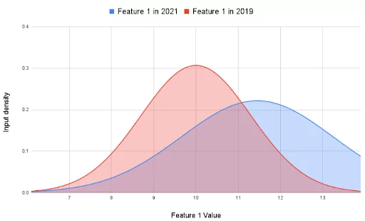
Another scenario that represents the seasonality in the data is illustrated in the image below. It shows how a data feature can change over the span of two years.

Target drift

Target drift occurs due to the shift in the numerical or categorical outcomes of the model. The addition or deletion of new classes in the dataset can result in target drift. While retraining can help measure the model decay caused by the drift, early identification of the changes in the classes or the data design can help avoid it.

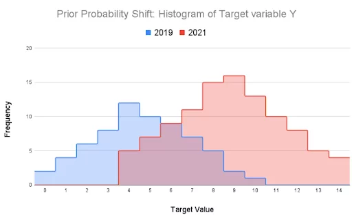
Consider the scenario in the image below where company X hadn’t experienced any financial loss during the Covid lockdown (2019-2021) and decided not to return the loan installments and take advantage of the government subsidy. Following the plan, the company saved more money (Y) to tackle any deteriorating circumstances. The distribution of the input variable remained the same, whereas the target variable Y changed.

Concept drift

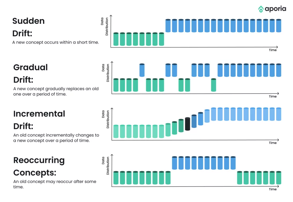
When the patterns on which the model was trained change, it leads to concept drift that affects the model’s accuracy and eventually makes it outdated. Concept drift can be gradual, where the model degrades without incorporating the changing needs over time. 

Moreover, abrupt drift occurs due to sudden changes in behavior or events. Such as a sudden increase or decrease in particular product demand during a certain period. Remember the “Great Toilet Paper” shortage during Covid? Finally, concept drift can happen periodically due to the repetition of events. For instance, customer buying patterns spike during holidays or festivals.

How to calculate statistical distribution drift?

Distribution drift, particularly data drift, can be identified using statistical techniques. It involves calculating the difference between training features and production features. In statistics, you have numerous techniques that can measure this difference in terms of the distance between the distributions of two attributes, some of which are:  

• Kolmogorov–Smirnov Test (K-S)
• Wasserstein Distance
• Population Stability Index (PSI)
• Cramér-von Mises (CM) distance

The details of each of these techniques are out of this article’s scope. However, we have added a brief code snippet below that demonstrates how the K-S test can be implemented for two attributes (one representing training data attribute and one representing production data attribute) using Python’s scipy library. 

# import relevant library
from scipy import stats
# size of training data attribute
n1 = 100  
# size of production data attribute
n2 = 200 
# define two random variates. One for training data (tdrv) and one for production data (pdrv) attributes 
tdrv = stats.norm.rvs(size=n1, loc=0., scale=1, random_state=0)
pdrv = stats.norm.rvs(size=n2, loc=0.5, scale=1.5, random_state=0)
# call the ks_2samp() method on the two random variates which returns the K-S statistic and pvalue for the two observations
stats.ks_2samp(tdrv, pdrv)

Output:

Ks_2sampResult(statistic=0.25, pvalue=0.0004277461336584798)

Adjust the loc and scale of the two random variates to get different distributions every time. Observe the resulting p-value for each experiment to figure out how similar or different the two distributions are.

How to use Aporia to evaluate model performance in production?

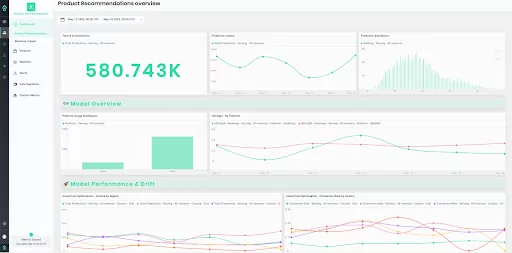
Aporia’s ML observability platform provides detailed model performance evaluation in production for every model and any use case. Within the platform, you can create dashboards to visualize the performance metrics of your models, set alerts to notify you of any significant changes or anomalies in these metrics, and use Aporia’s various features to investigate and debug any issues you may encounter. You can enable priority-based alerts, monitor custom metrics, observe data stats, and visualize model performance.

This way, Aporia allows you to continuously monitor your ML models and ensure that they are performing as expected, providing valuable insights into their behavior and assisting in their continual improvement. 

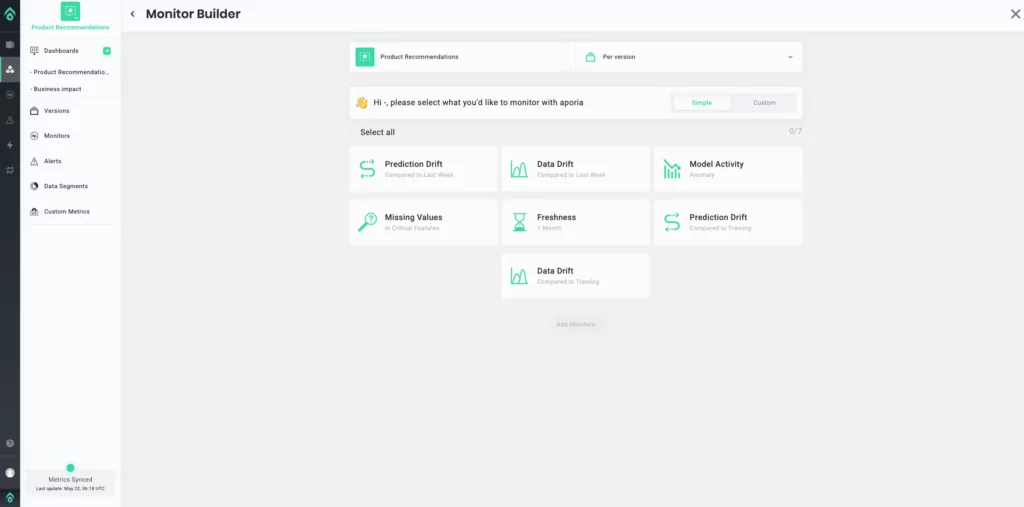
Aporia Monitor Builder allows ML teams to create “Simple” and “Custom” ML model monitoring pipelines that can track various model activities, prediction drift, data drift, F1 score, missing values, and more. The “Simple” Monitor Builder offers pre-defined monitoring options.

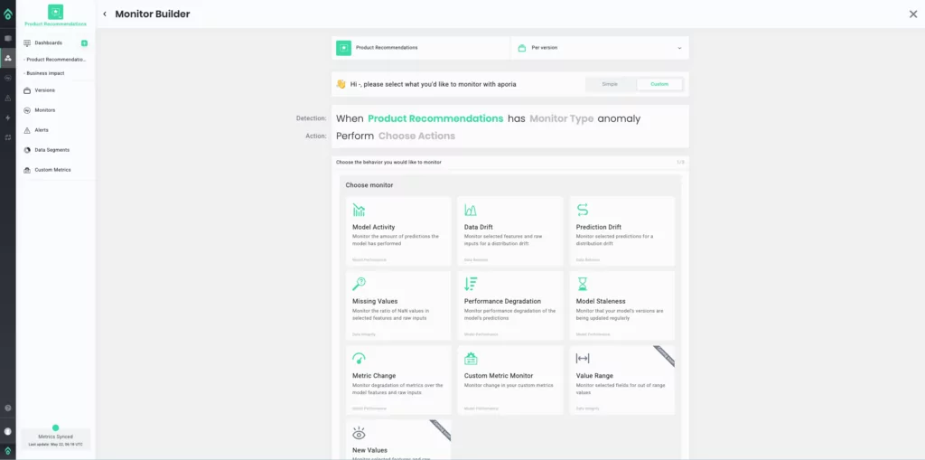
The “Custom” option offers a range of monitoring activities and allows the ML team to define any set of metrics for any features and generate alerts based on their desired metric threshold values.

Want to learn more about Aporia’s fit in your ML stack, book a demo with one of our ML observability experts.

Gon Rappaport