

February 29, 2024 - last updated
Drift Metrics
A practical introduction to Population Stability Index (PSI)
Managing model drift in practical machine learning applications is critical: As real-world data continually transforms, a model based on past data is likely to experience a decline in accuracy, leading to suboptimal decisions and potential financial impacts for the enterprise that depends on the model’s output.
Imagine you’ve developed a credit-scoring model for the financial industry to assess the creditworthiness of potential borrowers. You developed the model using historical data that encompasses a plethora of attributes including credit history, income, outstanding debts, and repayment behavior. But as the economy and the credit market have evolved, borrower profiles, risk factors, and repayment patterns have changed dynamically. If you don’t update the credit-scoring model based on these changes, your model may make inaccurate risk assessments, which could lead to elevated default rates and severe financial losses for your client.
What is Population Stability Index (PSI)
The Population Stability Index (PSI) is a statistical measure rooted in information theory, assessing the distinction between a given probability distribution and a reference distribution.
Tracking model drift with PSI
The Population Stability Index (PSI) is a valuable and often underutilized metric for assessing the stability of a model’s performance. PSI, a numerical marker, excels at detecting distributional shifts in data between a model’s training dataset and a newer one, often showcasing more recent data. By identifying changes in input parameter distribution and target variable, PSI provides data scientists and engineers with actionable insights into the performance and relevance of their data-centric solutions. Incorporating PSI into regular machine learning model assessments allows organizations to swiftly uncover model drift and implement required adjustments to ensure the reliability and efficacy of their models’ performance.
In our credit-scoring example, PSI is pivotal in identifying discrepancies between the credit-scoring model’s assumptions and the actual data. A model developed during a period of economic prosperity might misjudge the risk of default during a recession when unemployment rates skyrocket and borrowers find it difficult to repay their loans. You can use the PSI metric to compare the distribution of credit scores in the dataset you used to build the model and a more recent validation dataset to gauge the divergence between the two datasets.
A significant surge in PSI implies a substantial shift in the fundamental data, which makes the credit-scoring model less reliable. It’s imperative to reassess and reevaluate the model using more recent data that better reflects the current economic conditions and borrower profiles so that the model makes more accurate risk assessments and your organization can make informed lending decisions, safeguarding financial stability.
PSI in model monitoring
PSI plays a pivotal role in model monitoring by serving as an early warning system for model drift. As data evolves over time, the PSI metric can identify significant changes in the underlying distribution that may compromise the model’s predictive accuracy. By regularly computing PSI for key variables, you can proactively identify when a model might need retraining or adjustment. Despite its limitations, PSI is a simple, computationally efficient tool that complements other model monitoring techniques, helping maintain the integrity and reliability of your machine learning models in a dynamic data landscape.
Understanding PSI: Mathematical and intuitive explanations
An Intuitive Explanation:
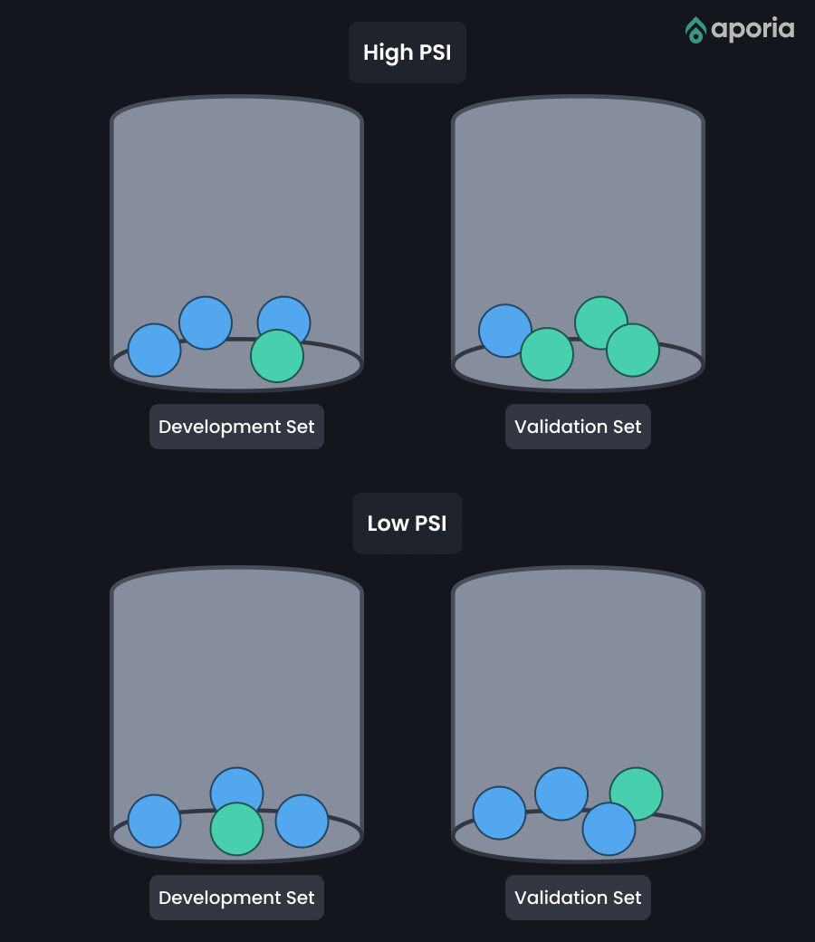
Imagine a jar filled with multi-colored marbles. Each color symbolizes a category, for example, credit risk level. To craft a model, you grab a handful of marbles (the development set). To assess the model, you take another handful (the validation set). If you were to place each of these two sets of marbles in a new jar and compare them, a similar balance of colors between the jars would mean a low PSI and the model is stable. If there is significant color variation between the jars, there is a high PSI, which is cause for concern.
A Mathematical Explanation:
- Partition
- Partition your dataset into categories (or bins) based on the predicted variable or score. Deciles are often used for this purpose.
- Compute the proportion of observations in each category for the development population (P_dev) and the validation population (P_val).
- Calculate the PSI for each category
- For each category, calculate the PSI with this formula:
PSI = (P_val – P_dev) * ln(P_val / P_dev)
- Get the overall PSI
- Add up the PSI values for all categories to get the overall PSI.
Formula Breakdown:
- P_dev and P_val: These proportions represent the observations in each category for the development and validation populations. Here’s how you can calculate them:
P_dev = (Number of observations in the category in the development set) / (Total number of observations in the development set)
P_val = (Number of observations in the category in the validation set) / (Total number of observations in the validation set)
- ln(P_val / P_dev): The natural logarithm of the P_val to P_dev ratio captures the divergence between the proportions. A zero value indicates no divergence, while increasing values signal growing dissimilarity.
- (P_val – P_dev) * ln(P_val / P_dev): This mesmerizing product measures the degree of divergence between the development and validation populations in each category.
- Overall PSI: Summing the PSI values for all categories provides the overall PSI. A high PSI warns of an unstable model, while a low PSI indicates stability.
PSI Value Interpretation:
- PSI < 0.1: Insignificant change—your model is stable!
- 0.1 <= PSI < 0.25: Moderate change—consider some adjustments.
- PSI >= 0.25: Significant change—your model is unstable and needs an update.
PSI evaluates model stability by comparing category distributions in development and validation populations. Understanding PSI’s mathematical essence empowers analysts to effectively evaluate and maintain their models’ performance over time.
An example of PSI
Let’s take this dataset as a tool for demonstration.
# Development dataset
dev_data = pd.DataFrame({'score': [15, 20, 25, 30, 20, 15, 10, 5, 30, 10]})


# Validation dataset
val_data = pd.DataFrame({'score': [15, 20, 24, 25, 20, 15, 10, 5, 30, 10]})
Step 1: Create bins for the data
Let’s create 5 bins for the given data which will result in a different PSI value but make it easier to demonstrate. The bins can be created based on the range of the ‘score’ variable:
- Bin 1: [0-9]
- Bin 2: [10-19]
- Bin 3: [20-29]
- Bin 4: [30-39]
- Bin 5: [40-49]
Step 2: Calculate the percentage of observations in each bin for both datasets
Development dataset (Dev):
- Bin 1: 1/10 = 0.1
- Bin 2: 3/10 = 0.3
- Bin 3: 3/10 = 0.3
- Bin 4: 2/10 = 0.2
- Bin 5: 0/10 = 0
Validation dataset (Val):
- Bin 1: 1/10 = 0.1
- Bin 2: 3/10 = 0.3
- Bin 3: 4/10 = 0.4
- Bin 4: 1/10 = 0.1
- Bin 5: 0/10 = 0
Step 3: Calculate the PSI using the formula
PSI = Σ (dev% – val%) * ln(dev% / val%)
For each bin, calculate the PSI component and sum them up:
- Bin 1: (0.1 – 0.1) * ln(0.1 / 0.1) = 0
- Bin 2: (0.3 – 0.3) * ln(0.3 / 0.3) = 0
- Bin 3: (0.4 – 0.3) * ln(0.4 / 0.3) ≈ 0.111226
- Bin 4: (0.1 – 0.2) * ln(0.1 / 0.2) ≈ 0.079441
- Bin 5: Since both Dev% and Val% are 0, the PSI component is 0.
Now, sum up the PSI components:
PSI = 0 + 0 + 0.111226 + 0.079441 + 0 = 0.190667
The PSI for the given data sets is approximately 0.190667. Keep in mind that in practice, you may want to use more or less bins depending on your data.
Implementing PSI
For the sake of this walkthrough, we will be using the following libraries:
import numpy as np
import pandas as pd
import matplotlib.pyplot as plt
If you are missing any of the libraries, you can install them with the following commands:
pip install numpy
pip install pandas
pip install matplotlib
We will be focusing on two datasets, which we will create for the sake of demonstration:
Development dataset
In the initial stages of model building, the development dataset is used for data exploration, feature engineering, and model training, so that the model can capture the underlying patterns and relationships in the data. When calculating PSI, we use the development dataset as a reference or baseline.
Validation dataset
We use an independent dataset that is not used during the model training process—the validation dataset—to assess the performance of the model on unseen data to ensure that the model generalizes well to new instances.
When calculating PSI, we use the validation dataset to compare its distribution of the variable or score against the development dataset. A significant change in the distribution may indicate a shift in the underlying population or the presence of external factors that were not captured during the model development process.
# Development dataset
dev_data = pd.DataFrame({
    'score': [15, 20, 25, 30, 20, 15, 10, 5, 30, 10]
})


# Validation dataset
val_data = pd.DataFrame({
    'score': [15, 20, 24, 25, 20, 15, 10, 5, 30, 10]
})
Calculating PSI
Our workflow will look like this:
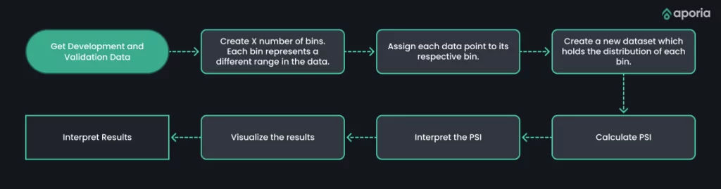
Now let’s create a method to calculate the PSI. The header will take the following parameters:
def population_stability_index(dev_data, val_data,col_name, num_bins=10):We pass the development data, the validation data, the column name, and the number of bins we will use. The number of bins is a parameter for the partitioning of a continuous variable, such as scores, into distinct intervals or categories. By designating the number of bins, you can effectively modulate the intricacy of the analysis when assessing the Population Stability Index (PSI).
For instance, imagine you’re working with scores that span from 0 to 100, and you decide to use 10 bins. In this case, each bin would correspond to a range of 10 units, such as 0-10, 10-20, 20-30, and so forth.
By creating bins and assigning each score to a bin, we can create a new categorical variable that represents the distribution of scores in each dataset. This categorical variable can be used to compare the distribution of scores between the two datasets.
The next line calculates the minimum and maximum scores in the development dataset and creates num_bins + 1 equally spaced bin edges.
bins = np.linspace(dev_data[col_name].min(), dev_data[col_name].max(), num_bins + 1)Next, we assign each score in both datasets to the corresponding bin. “pd.cut” is a pandas function that categorizes a continuous variable into discrete bins based on specified edges.
dev_data['bin'] = pd.cut(dev_data[col_name], bins=bins, include_lowest=True)
val_data['bin'] = pd.cut(val_data[col_name], bins=bins, include_lowest=True)
We group the data by bins, and the number of scores in each bin is counted for both datasets. The result is stored in two separate data frames, dev_group and val_group.
dev_group = dev_data.groupby('bin')[col_name].count().reset_index(name='dev_count')
val_group = val_data.groupby('bin')[col_name].count().reset_index(name='val_count')
The next line merges the dev_group and val_group data frames based on the ‘bin’ column. The ‘left’ join ensures that all bins from the development dataset are included in the final merged data frame, even if there are no scores in the validation dataset for those bins.
merged_counts = dev_group.merge(val_group, on='bin', how='left')Next, we calculate the PSI value for each bin. First, a small constant is added to both the development and validation percentages to avoid division by zero. Then the percentage of scores in each bin is calculated for both datasets. Finally, the PSI is calculated for each bin using the formula (val_pct – dev_pct) * log(val_pct / dev_pct).
small_constant = 1e-10
merged_counts['dev_pct'] = (merged_counts['dev_count'] / len(dev_data)) + small_constant
merged_counts['val_pct'] = (merged_counts['val_count'] / len(val_data)) + small_constant
merged_counts['psi'] = (merged_counts['val_pct'] - merged_counts['dev_pct']) * np.log(merged_counts['val_pct'] / merged_counts['dev_pct'])
Lastly, we return the sum value of all the bins.
return merged_counts['psi'].sum()If we run the method we just created, we get the following output with a PSI Value of 0.14.
psi_value = population_stability_index(dev_data, val_data, 'score')
print(f"PSI Value: {psi_value}")
A PSI value of 0.14 is considered a bit concerning, an accepted rule of thumb is that a change of about 0.2 or higher is cause for concern.
| PSI Value | Description |
| PSI < 0.1 | Very low change between the two groups, considered stable. |
| 0.1 <= PSI < 0.25 | High change between the two groups, is considered significant. |
| PSI >= 0.25 | High change between the two groups, considered significant. |
PSI visualization
To visualize the PSI, we will create a prepare_data_for_plotting method that functions similarly to the population_stability_index. Instead of calculating the PSI, this method will populate two extra columns with the percentages of each bin. To format the information so that it’s easier for people to understand, we will multiply the percentage by 100.
def prepare_data_for_plotting(dev_data, val_data, col_name, num_bins=10):
    bins = np.linspace(dev_data[col_name].min(), dev_data[col_name].max(), num_bins + 1)

    dev_data['bin'] = pd.cut(dev_data[col_name], bins=bins, include_lowest=True)
    val_data['bin'] = pd.cut(val_data[col_name], bins=bins, include_lowest=True)


    dev_group = dev_data.groupby('bin')[col_name].count().reset_index(name='dev_count')
    val_group = val_data.groupby('bin')[col_name].count().reset_index(name='val_count')


    # Merge dev and val counts
    merged_counts = dev_group.merge(val_group, on='bin', how='left')

    # Calculate percentages
    merged_counts['dev_pct'] = merged_counts['dev_count'] / len(dev_data) * 100
    merged_counts['val_pct'] = merged_counts['val_count'] / len(val_data) * 100


    return merged_counts
Now we can create a basic plot function.
def plot_psi(dev_data, val_data, psi_value, col_name):
    plot_data = prepare_data_for_plotting(dev_data, val_data,col_name)


    fig, ax = plt.subplots(figsize=(15, 8))  # Adjust the chart size here
    index = np.arange(len(plot_data))
    bar_width = 0.35


    dev_bars = ax.bar(index, plot_data['dev_pct'], bar_width, label='Development')
    val_bars = ax.bar(index + bar_width, plot_data['val_pct'], bar_width, label='Validation')

    ax.set_xlabel('Bins')
    ax.set_ylabel('Percentage')
    ax.set_title(f'Population Stability Index (PSI): {psi_value:.4f}')
    ax.set_xticks(index + bar_width / 2)
    ax.set_xticklabels(plot_data['bin'].apply(lambda x: f"{x.left:.2f}-{x.right:.2f}"))
    ax.legend()


    fig.tight_layout()
    plt.show()
Finally, we can call the plot_psi function to visualize the change.
plot_psi(dev_data, val_data, psi_value)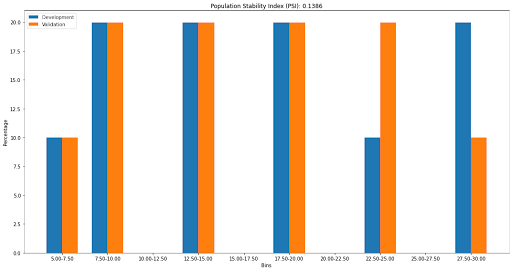
Our bar chart shows a slight change in the 22.5-25 and 27.5-30 bins, but the change isn’t large enough to warrant concern.
Comparing PSI to alternative approaches
Although PSI is not the only technique for detecting model drift, it is a popular metric for measuring a model’s stability for its simplicity, ease of interpretation, and applicability to both categorical and continuous variables. Calculating PSI is quick, requires minimal computational resources, and is easily understood by non-experts. Additionally, PSI works with various data types, making it adaptable across many machine learning applications.
However, PSI has limitations. First, PSI only measures drift in a single variable’s distribution, possibly overlooking complex interactions or dependencies between variables. Second, PSI is sensitive to binning choices, as inappropriate binning may produce inaccurate or misleading results. Third, PSI cannot distinguish between different types of drift, such as concept drift, data drift, or label drift, each requiring a unique mitigation strategy.
Other model drift detection methods include statistical tests like the Kolmogorov-Smirnov test, Kullback-Leibler divergence, and Wasserstein distance, which also measure the divergence between reference and new dataset distributions but provide a more complete drift assessment. These tests are more complex, computationally demanding, and difficult to interpret, so they may not be practical in all cases.
Another approach to detecting model drift is to monitor a model’s performance on a validation set over time using metrics such as accuracy, precision, recall, or the F1 score. This method gives a direct measure of model performance but might be less sensitive to subtle changes in data distribution or detect drift only after it has negatively impacted performance.
No single method is universally suitable for detecting model drift. Instead, a combination of techniques may be more effective. For instance, PSI could be used as an initial screening tool to identify potential drift, followed by more advanced tests or performance monitoring for further investigation.
Calculating PSI with Aporia
Aporia’s ML Observability platform provides a comprehensive suite of metrics to understand and monitor your machine learning models in production, and one such important metric it supports is the Population Stability Index (PSI).
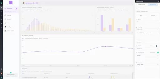
Within the Aporia platform, calculating PSI is straightforward and intuitive. Aporia automatically calculates the PSI for selected features and raw inputs across different time frames, model versions, and data segments. You can then visualize this information on your custom dashboards, allowing you to monitor drift and model stability in real-time. If there are substantial shifts in the feature distribution, Aporia’s monitoring system can trigger alerts, enabling you to quickly respond to any potential issues. This makes the process of tracking model stability and detecting drift a seamless part of your ML workflow.
Conclusion
As data distributions inevitably shift over time, PSI is a valuable tool for identifying and controlling model drift and ensuring the accuracy and effectiveness of your machine learning application. Despite its limitations, PSI is a sturdy and adaptable technique that can be used alongside other drift monitoring methods to ensure the optimal performance of your model in a swiftly changing data environment.
Book a demo to see how Aporia uses PSI.
