Understanding embeddings in machine learning: Types, alternatives, and drift

Introduction

Machine learning algorithms, specifically in NLP, LLM, and computer vision models, often deal with high-dimensional and unstructured data, such as text or images, which can be difficult to work with directly. Embeddings are a technique used in machine learning to reduce the dimensionality of data and represent it in a more meaningful way. 

In this post, we’ll introduce embeddings and explain how they are created, the types of embeddings, how to use pre-trained embeddings, alternatives to embeddings, and how to evaluate them.

What are embeddings?

Embeddings are a technique for representing high-dimensional data in a lower-dimensional space. They are typically represented as vectors, where each element of the vector corresponds to a feature of the data. Once the model is trained on some task, the values of the model’s parameters are used as the embeddings for the data. Embeddings are useful because they capture the underlying structure of the data in a way that is more meaningful than simply representing the data as a set of features. For example, in natural language processing (NLP), embeddings can be used to represent words in a way that captures their semantic relationships.

Types of embeddings

There are several types of embeddings, each designed for a specific type of data. Some common types of embeddings include:

• Word embeddings: used in natural language processing (NLP) to represent words as vectors.
• Image embeddings: used in computer vision to represent images as vectors.
• Graph embeddings: used in network analysis to represent graphs as vectors.

Each type of embedding has its own properties and techniques for creating them. Throughout this guide, we’ll focus on the first two embeddings, which are most commonly used. 

Training embeddings from scratch

To create embeddings from scratch, we first need to choose a machine learning algorithm to use. One popular algorithm for creating embeddings is the neural network. A neural network is a machine learning model that consists of layers of interconnected neurons, each of which performs a simple computation on its inputs.

To create embeddings using a neural network, we can train the network to predict the values of the features, given the data. Once the network is trained, the values of the weights of the network’s layers can be used as the embeddings.

The word2vec algorithm is used to train a model for text embeddings. It uses a CBOW or skip-gram objective. CBOW stands for continuous bag-of-words and is executed by predicting a word given a context window of 2k-1 words.

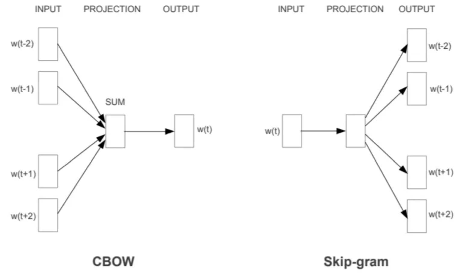
 For example in CBOW, when k=2, for the text “I love to eat chocolate” the following training samples and targets would be created, the targets are marked with <>. 

1. I <love> to
2. love <to> eat
3. to <eat> chocolate

To train this model, it is possible to use the gensim implementation of the word2vec model:  

from gensim.models import Word2Vec

documents = ['First, this is the first sentence.',
             'And this is the second.',
             'Is this the third sentence?']

documents = [
        [word.lower() for word in doc.split()] for doc in documents]


model = Word2Vec(documents, min_count=1)

print(model.wv["first"])

Using pre-trained embeddings

While creating embeddings from scratch is a powerful approach, it can be time-consuming and requires a large amount of data. Alternatively, pre-trained embeddings can be used. Pre-trained embeddings are embeddings that have already been trained on a large dataset and can be used as a starting point for a machine-learning model.

Pre-trained embeddings have been trained on massive datasets and can capture many of the relationships between the features in the data. Using pre-trained embeddings can help improve the accuracy of machine learning models and reduce the time and resources required for training.

The output of Word2Vec is a set of embeddings, where each embedding represents a word in the vocabulary. Word2Vec is trained on large text corpora, such as Wikipedia or news articles, and captures many of the semantic relationships between words.

Here’s an example of how to use pre-trained embeddings in Python using gensim:

import gensim.downloader as api
wv = api.load('word2vec-google-news-300')
vec_first = wv['first']
print(vec_first)

But, as mentioned before, embeddings can be obtained for images too. Here’s an example of how to use pre-trained embeddings using HuggingFace ViT (vision transformers):

from transformers import ViTFeatureExtractor, TFViTForImageClassification
import tensorflow as tf
from PIL import Image
import requests


url = "http://images.cocodataset.org/val2017/000000039769.jpg"
image = Image.open(requests.get(url, stream=True).raw)


feature_extractor = ViTFeatureExtractor.from_pretrained("google/vit-base-patch16-224")
model = TFViTForImageClassification.from_pretrained("google/vit-base-patch16-224")


inputs = feature_extractor(images=image, return_tensors="tf")
outputs = model(**inputs)
logits = outputs.logits
# model predicts one of the 1000 ImageNet classes
predicted_class_idx = tf.math.argmax(logits, axis=-1)[0]
print("Predicted class:", model.config.id2label[int(predicted_class_idx)])


# Output: Predicted class: Egyptian cat

Using pre-trained embeddings isn’t confined to just computer vision and NLP models; it extends profoundly into the land of Large Language Models (LLMs) and Generative AI. These LLMs, often trained on enormous datasets, leverage embeddings to comprehend linguistic nuances and generate coherent, contextually relevant outputs.

An alternative to embeddings

One-Hot Encoding

Embeddings are a powerful technique in machine learning, but alternatives do exist. One such is one-hot encoding, which represents categorical data as binary vectors. Each element of the vector represents a possible category, and the value of the element is 1 if the data point belongs to that category and 0 otherwise.

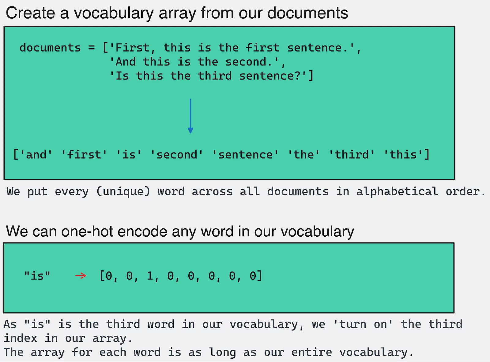
This example demonstrates how to perform one-hot encoding on a dataset with a single column ‘document’. It transforms the text data into a binary vector where each unique word gets its own column.

import pandas as pd

# Suppose we have a simple dataset
data = {'document': ['and', 'is', 'first']}
df = pd.DataFrame(data)

# One-hot encode the 'document' column
df_encoded = pd.get_dummies(df, columns=['document'])

print(df_encoded)

The function pd.get_dummies() is used to convert the categorical variable into dummy/indicator variables. The parameter columns=['document'] specifies that we want to perform the one-hot encoding on the ‘document’ column.

The output df_encoded is a DataFrame where each unique fruit from the ‘document’ column is represented as its own column in the DataFrame. A row will have a 1 under the column for the word it represents and 0 under all other columns.

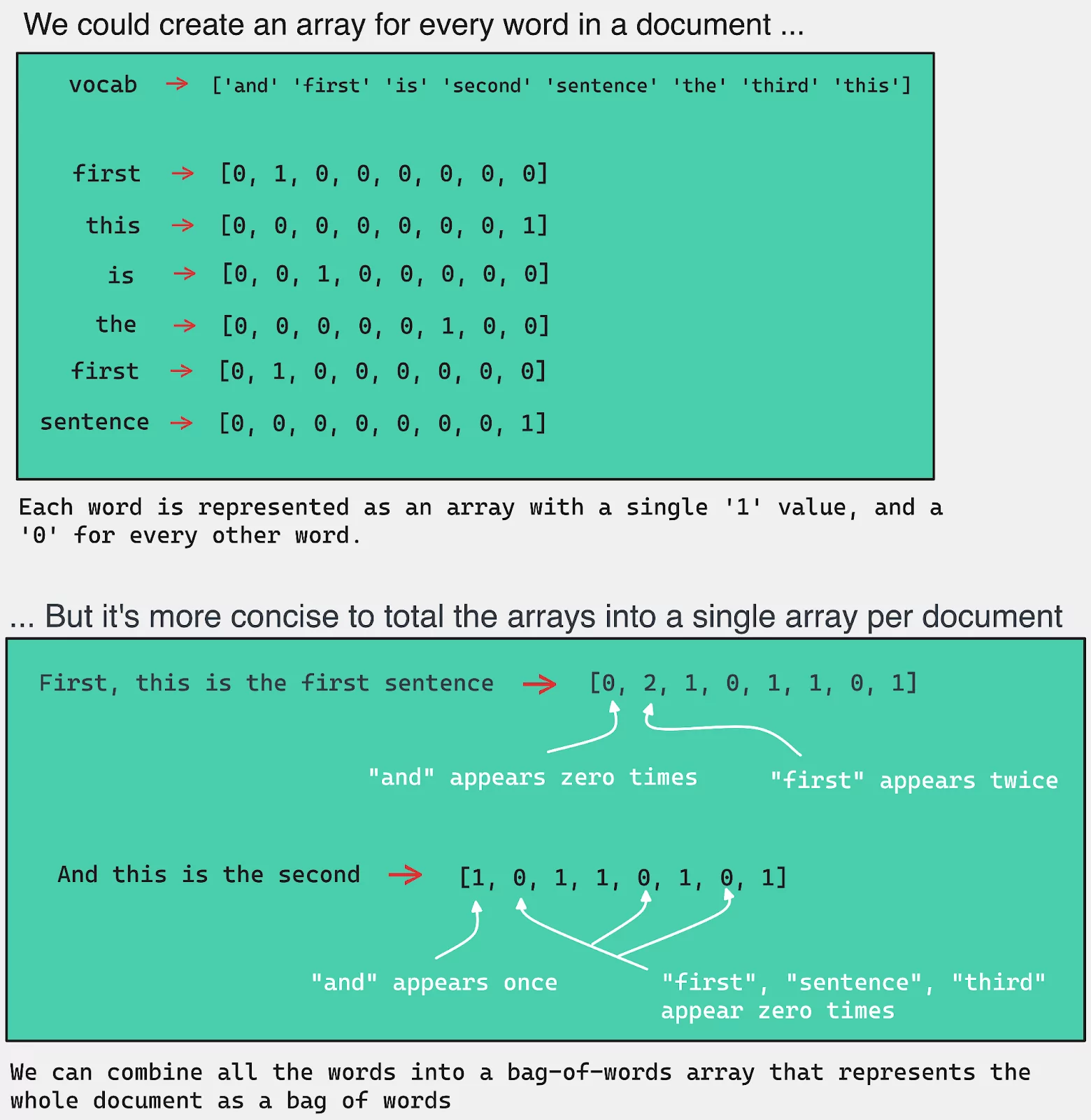
Bridging One-Hot Encoding with Bag-of-Words

To further extend the utility of one-hot encoding, we can explore the Bag-of-Words (BoW) model, especially in the context of natural language processing (NLP). While one-hot encoding provides a binary representation, the BoW model offers a representation based on word counts, retaining the frequency of words in a document but ignoring their order. This means, that in addition to knowing the presence of words (as in one-hot encoding), we can understand their prevalence in the document, providing more nuanced information.

This is a simpler and more discrete approach than the continuous bag of words (CBOW) we presented before. The idea is to represent a document as a bag of words, where the order of the words is ignored, and only the frequency of the words is retained.

This code illustrates how to transform a list of sentences into a bag-of-words representation using the CountVectorizer class from the Scikit-learn library.

from sklearn.feature_extraction.text import CountVectorizer

# Let's take a list of sentences
documents = ['First, this is the first sentence.',
             'And this is the second.',
             'Is this the third sentence?']

# Create a CountVectorizer instance
vectorizer = CountVectorizer()

# Learn and count the words in 'documents'
bag_of_words = vectorizer.fit_transform(documents)

# Check the result
print(vectorizer.get_feature_names_out())
print(bag_of_words.toarray())

# Output
# [[0 2 1 0 1 1 0 1]
#  [1 0 1 1 0 1 0 1]
#  [0 0 1 0 1 1 1 1]]

The CountVectorizer class converts a collection of text documents (in this case, the ‘documents’ list) to a matrix of token counts. The method fit_transform() learns the vocabulary dictionary (all the unique words across all documents) and returns a matrix where each row corresponds to a document and each column corresponds to a word from the vocabulary. The value in each cell is the count of a word in a particular document.

The output of vectorizer.get_feature_names_out() is an array of feature names (the words), and bag_of_words.toarray() converts the sparse matrix to a regular (dense) NumPy array, which is easier to read and understand.

Choosing A technique

The choice of technique depends on the type of data and the task at hand. Embeddings are useful when the relationships between the features are important, while one-hot encoding and bag-of-words models are useful when the categorical nature of the data is important. 

These methods are hard to manage and linearly scale according to the vocabulary/data size, and the embedding method is aimed to address these disadvantages.

Detecting embeddings drift

Analyzing unstructured data drift is essential to detect whether two datasets or splits differ. It requires a deeper understanding of the underlying relationships within the data itself – it is necessary to gain a comprehensive understanding of the data in order to detect and measure it.

With the rise of LLMs, embedding drift can potentially influence the model’s ability to generate accurate and reliable outputs, resulting in garbage responses or hallucinations. Implementing LLM observability and monitoring is vital in tracking embedding drift. This ensures the efficiency and reliability of LLMs, especially when the models are constantly evolving and adapting to new data.

What does drift look like?

When the model training data is not sufficient and not robust to variations, data drift can occur. Some variations can be different perspectives, lighting conditions, and other factors that can affect image appearance or different syntax, semantics, and linguistic nuances and vocabulary in NLP.

Detecting drift in unstructured data

Detecting drift in unstructured data can be challenging, but one effective approach is to use embedding vectors to lower the dimensionality of the data while retaining its key semantic features and connections. By comparing the embeddings of the data at different time periods or in different data splits, we can detect and measure any significant shifts in the distribution or characteristics of the data, which may indicate drift. Therefore, the use of embedding vectors is a valuable technique for model monitoring and detecting drift in unstructured data.

Techniques for detecting embedding drift

To detect drift in embeddings, we can use various techniques that compare pre-trained embeddings with new embeddings. Two common methods include cosine similarity/distance and Euclidean distance.

1. Comparison of pre-trained embeddings with new embeddings using cosine similarity/distance:

• Cosine similarity/distance: This measures the cosine of the angle between two vectors and indicates the similarity between embeddings. A cosine similarity closer to 1 indicates higher similarity, while a value closer to -1 indicates lower similarity. The cosine distance can be calculated as 1 minus the cosine similarity.

from sklearn.metrics.pairwise import cosine_similarity

embedding1 = ...
embedding2 = ...
similarity = cosine_similarity([embedding1], [embedding2])[0][0]
distance = 1 - similarity

2. Euclidean distance: This method measures the straight-line distance between two vectors and can capture changes in embeddings. Larger Euclidean distances indicate a greater difference between the embeddings.

from scipy.spatial.distance import euclidean

embedding1 = ...
embedding2 = ...
distance = euclidean(embedding1, embedding2)

Embeddings visualization techniques

Visualization techniques such as PCA, t-SNE, and UMAP can also be used to detect drift in embeddings.

1. PCA (Principal Component Analysis): A linear dimensionality reduction technique that can help visualize high-dimensional embeddings in a 2D or 3D space.
2. t-SNE (t-Distributed Stochastic Neighbor Embedding): A non-linear dimensionality reduction technique that is particularly useful for visualizing high-dimensional data.
3. UMAP (Uniform Manifold Approximation and Projection): A non-linear dimensionality reduction method that is faster than t-SNE and can handle larger datasets.

Mitigating embedding drift

Consider implementing these methods to reduce drift impact:

1. Regularly update pre-trained embeddings with new data to capture the evolving relationships between data points.
2. Monitor model performance and perform drift detection analysis to identify shifts in embeddings.
3. Use data augmentation techniques to increase the robustness of the model to variations in the input data.
4. Combine multiple embedding techniques or models to improve generalization and reduce the impact of drift on individual embeddings.
5. Implement active learning strategies to selectively obtain new training data that addresses the changes in data distribution.

Wrapping up 

Embeddings play a pivotal role, offering a gateway to efficiently analyze high-dimensional data found in text or image analytics. This guide unpacked the nuances of various embeddings, including text and image, and illustrated the merits of utilizing pre-trained models, promoting heightened linguistic comprehension and output relevance.

However, the journey doesn’t end here. It is crucial to navigate potential embedding drifts that could hamper the effectiveness of LLMs. By adopting stringent ML observability protocols, you can monitor and counteract these drifts, ensuring your AI models not only adapt to changing data landscapes but do so responsibly, with unwavering accuracy and reliability.

Want to learn more about monitoring visualizing, and exploring unstructured data? Reach out to us for a guided tour on monitoring embeddings or jump into the Aporia platform and try it out yourself. 

Niv Hertz